Species Beta diversity

distance and similarity

Any statistical result that satisfies nonnegative, reflexive and trigonometric inequalities can be called distance. Distance is used to describe the distance of two statistical objects ^[1]. The object can be a community of one or more points on the axis. the greater distance represents the greater difference between objects

When two objects have more similar attributes, the more similar the two objects are. For example, the number and length of edges of regular polygons are two attributes, if the number of edges of two regular polygons is equal, then they are similar, if the number and length of edges are equal, then they are all equal. For the two communities, the Species composition of the community is their attribute. The more the number of Species shared by the two communities, the closer the relative abundance of the commonSpecies, and the greater the similarity between the two communities. Similarity is described by similarity index. the higher similarity index represents the more similar sample.

to be paid attention

All similarity indices can be converted into corresponding distances, but not all distances can be converted into similarity indices.

The essence of beta diversity

Beta diversity ^[2] uses the abundance information (gene, species or function) of each sample to calculate the distance or similarity between samples, and reflects whether there are significant microbial community differences among samples (groups) or habitats (between-habitat diversity) through distance, also known as inter-habitat diversity.

Simply, Beta diversity analysis focuses on the differences between samples.

Double zero problem

In microbial data, there is often a situation in which a microorganism is not detected in both samples, and the meaning of Species deletion (double zero data) determines whether it can be used as a basis for judging the similarity of the two samples. There are two situations:

• Neither of the sampling sites meets the survival conditions of the species, or the species has never spread here.
• The species was not included in the sample at the time of sampling, or the content of the species in the sample is too low and too low to be annotated.

Double zero data often appear in microbial ecology, if the meaning of double zero data is the same, then double zero data can be used as a basis to judge the similarity between the two. However, the Mega Genome Project itself is exploring an unknown environment, so it is usually impossible to determine whether the meaning of double zero data is the same in different samples, and with the increase of the number of Species, the probability of double zero data between samples increases, and this uncertainty is also increasing.

Symmetry and asymmetry are used to describe the above double zero problem, if the meaning of double zero data is the same, it can be used as the basis for judging similarity, which is called symmetry, otherwise it is asymmetry. In most cases, asymmetry should be preferred unless it can be determined that zero data has the same meaning.

Beta diversity measurement

Metagenomics project usually adopts Euclidean distance ^[3](Euclidean distance), Bray - Curtis phase heterosexual index (Bray - Curtis Distance) ^[4]（Bray-curtis distance）and JSD distance (Jensen - Shannon divergence) to measure the difference between the sample (group). It is the basis of Beta diversity analysis to calculate the distance between multiple samples and place the distance information in the table to form a distance matrix.

here

The Euclidean distance is symmetric (double zero data have the same meaning), and the other two are asymmetric. Therefore, Euclidean distance should be used with caution when there are many zeros in the sample pair.

Euclidean distance

Euclidean distance is a distance often used in multivariate analysis, and its formula is as follows:

$$E_{ij}= \sqrt {\sum_{n}(S_{in} - S_{jn})^2}$$

$i$、$j$：two sample

$n$：n th item in sampleSpecies

$S_{in}$：$i$ Abundance of $n$th Species in the sample

$S_{jn}$：$j$ Abundance of $n$th Species in the sample

According to the formula, the Euclidean distance depends on the abundance of the input, and its value range is $[0, +\infty]$. The greater the Euclidean distance, the greater the difference between the two samples.

Bray-Curtis distance

Bray-Curtis distance is one of the most commonly used distances to calculate microbial abundance differences. However, Bray-Curtis' calculation method does not conform to the triangle inequality in the definition of distance, so it is not strictly a distance. The correct name is Bray-Curtis anisotropy index. This report also refers to it as the Bray-Curtis distance.

When calculating the Bray-Curtis distance, the samples that are not detected in either sample will be ignored. Its calculation formula is as follows:

$$BC_{ij} = 1-\frac{2C_{ij}}{S_i+S_j}$$

$i$、$j$：two sample

$C_{ij}$：Compare the abundance of each Speciesin the two samples and sum all the relatively low abundances of Species.

$S_i$：$i$ Sum of abundances of all Species in the sample

$S_j$：$j$ Sum of abundances of all Species in the sample

When using relative abundance data, the formula can be simplified to

$$BC_{ij} = 1-C_{ij}$$

According to the formula, the value range of Bray-Curtis distance is $[0, 1]$，When $BC=0$, it indicates that Speciescomposition of the two samples is completely consistent. $BC=1$ indicates that Species is not shared between the two samples. The smaller the BC value, the higher the similarity between the two samples and the smaller the difference.

JSD distance

JSD distance（Jensen–Shannon divergence，JSD divergence）is a distance index developed from KL divergence (Kullback–Leibler divergence) and used to describe the similar differences between two samples in probability distribution.

The JSD distance is also asymmetric, so samples that are not detected in either sample are ignored. The formula is as follows

$$JSD(P\parallel Q)= \frac{1}{2}D(P\parallel M) + \frac{1}{2}D(Q\parallel M)$$

where，the principles for calculating $M$ is

$$M = \frac{1}{2}(P+Q)$$

the principles for calculating $D$ is

$${D}(P\parallel Q)=\sum_{i} P(i)\ln \frac{P(i)}{Q(i)}$$

$P$：The abundance matrix for the first sample

$P(i)$：Abundance of $i$th Species in the first sample

$Q$：The abundance matrix of the second sample

$Q(i)$：Abundance of $i$th Species in the second sample

According to the formula, the value range of JSD distance is $[0, 1]$，The smaller the JSD value is, the higher the similarity between the two samples and the smaller the difference.

Beta diversity describes the differences between samples, using sample abundance data or similarity index and distance to describe. In the specific experiment, the difference between the grouping samples and whether the difference is significant or not is related to the effectiveness of the experimental grouping / application treatment, such as whether the use of a new type of filter material can significantly improve the community structure of attached bacteria compared with the filter material of the comparative group. so as to improve the metabolism of nitrogen and phosphorus in the filter.

However, whether it is abundance data or similarity and distance, Species component data belong to multivariate (multi-dimensional) samples. When we want to classify and visualize the high-dimensional data, we need to use the dimensionality reduction method to map the high-dimensional data to the two-dimensional plane or three-dimensional space, so that we can directly see the distance and similarity between different samples. According to the difference of data and statistical methods, the commonly used dimensionality reduction methods are PCA analysis, PLS-DA analysis, PCoA analysis and NMDS analysis. The comparison of them is as follows:

	PCA	PLS-DA	PCoA	NMDS
Name	Principal component analysis	Partial Least Squares Discriminant Analysis	Principal coordinate analysis	Non-metric Multidimensional Scaling
Whether to supervise	Without supervision	With supervision	-	-
Input data	abundance matrix	abundance matrix	distance matrix	distance matrix
Coordinate axis weight	Yes	Yes	Yes	No

Note：
Whether or not to supervise: with supervision, consider grouping; without supervision, do not consider grouping Coordinate axis weight: it is depended on whether the degree of interpretation of the coordinate axis to the variable is the same. If it is the same, the coordinate axis weight is considered, otherwise there is no coordinate axis weight.

PCA analysis

PCA ^[5] (Principal Components Analysis), also known as principal component analysis or principal component regression analysis. The idea of PCA dimensionality reduction is to first reduce the dimension of the data set, while maintaining the characteristics of the maximum contribution to the variance of the data set, and finally make the data intuitively presented in the two-dimensional coordinate system.

The main steps for PCA are as follows: （1）normalize the data.
（2）calculate the covariance matrix of the normalized data set.
（3）calculate the eigenvalues and Eigenvectors of the covariance matrix. （4）retain the most important k features (usually k less than n）；
（5）find out the corresponding eigenvectors of k eigenvalues.
（6）multiply the data set of m * n by * k * n*-dimensional Eigenvectors (n * k) to get the final reduced-dimensional data.

PLS-DA analysis

PLS-DA (PartialLeastSquaresDiscriminantAnalysis), partial least squares discriminant analysis, is a discriminant analysis method in multivariate data analysis, which is often used to deal with classification and discriminant problems. By properly rotating the principal components, PLS-DA can effectively distinguish the observations between groups, and can find the influence variables that lead to the differences between groups.

PLS-DA adopts the classical partial least squares regression model, and its response variable is a supervised discriminant analysis method, which is the classification information of the category relationship between a group of response statistical units. Because the unsupervised analysis method (PCA) does not distinguish all the samples, that is, each sample has the same contribution to the model, the unsupervised analysis method can obviously show the inter-group difference when the inter-group difference is large and the intra-group difference is small, while when the inter-group difference is not clear, but the intra-group difference is large, the unsupervised analysis method is difficult to find the inter-group difference. In addition, if the difference between groups is small, the sample size of each group varies greatly, and the group with large sample size will dominate the model. Supervised analysis (PLS-DA) can well solve these problems encountered in unsupervised analysis.

PCoA analysis

Multi-dimensional scale analysis ^[6]（Multidimensional scaling，MDS) (Multidimensional scaling,MDS) is an analysis method to visualize the sample location based on the dimensionality reduction of the similarity distance matrix between samples. PCoA is also called classical multi-dimensional scale analysis. The input matrices commonly used in PCoA analysis are Euclidean distance matrix, Bray-Curtis dissimilarity matrix, JSD divergence matrix and so on.

NMDS analysis

NMDS ^[7] (Non-metricMultidimensionalScaling) non-metric multidimensional scaling method is a data analysis method that simplifies the research objects (samples or variables) in multi-dimensional space to low-dimensional space for location, analysis and classification, while retaining the original relationship between objects. It is suitable for the situation where the accurate similarity or dissimilarity data between the research objects can not be obtained, but only the hierarchical relationship data between them can be obtained. The pros and cons of the NMDS results are defined by the stress coefficient (Stress value), which represents the difference between the distance between the point in the two-dimensional space and that in the multi-dimensional space. The calculation formula is as follows.

$$Stress = \sqrt{\frac{\sum(f(x)-d)^2}{\sum{d^2}}}$$

Normally when Stress ＜ 0.2 it can be represented by two-dimensional dot graph of NMDS, which has certain explanatory significance; when Stress < 0.1, it can be regarded as a good ranking; when Stress < 0.05, it has a good representation.

Statistical test

Statistical Test of Multidimensional data

Microbial community abundance data are multidimensional data, one of which Species represents a data dimension. The distance between samples can be expressed on a plane by dimensionality reduction, but whether they really have differences or not needs to be judged according to the statistical test results. The common situation is that the reduced-dimensional samples are marked on the two-dimensional plane, but there is a partial overlap between the samples of different groups. at this time, it is impossible to judge whether there is a difference between the groups in the diagram, which can only be judged by the statistical test results.

The statistical test of a dependent variable (one-dimensional) data is called (univariate) analysis of variance, which is based on the data itself. Similarly, the statistical test of high-dimensional data samples is called multivariate analysis of variance, which is based on the distance matrix, that is, multiple variables are first calculated according to different distance algorithms, and then the distance matrix is statistically tested.

Statistical tests are helpful to answer：

1. Does the change of independent variable (factor) have significant influence on dependent variable (experimental index)?
2. What is the relationship between dependent variables?
3. What is the relationship between independent variables?

Multivariate analysis of variance needs to meet the premise assumptions：

1. The sample data are independent of each other.
2. The data in each group conforms to the multivariate normal distribution.
3. The covariance matrix of the data in each packet is the same.

However, microbial community abundance data are often difficult to meet the above conditions, so the statistical test of microbial data is commonly used for multivariate nonparametric variance tests with no requirements for data distribution: Anosim and Adonis. They need to meet the premise that:

1. The data of each object is exchangeable.
2. Exchangeable objects (samples) are independent of each other.
3. The test data of each sample has a consistent multivariate distribution (the discreteness of each group of data is similar)

Zero hypothesis $H_0$：there is no difference in the central point (centroid) and dispersion (dispersion) of each group of samples in the detection space composed of their detection indexes, that is, there are differences between groups.

Both Adonis and Anosim are nonparametric statistical tests for multidimensional data, and both use the permutation test (the default number of permutations is 999). The difference is that the test model is different. Adonis is essentially based on the statistics of F and is often used with PCoA, while the statistic of Anosim is R, which is often used with NMDS.

When the p calculated by Anosim or Adonis is less than 0.05, accept the zero hypothesis and consider that there are differences between groups; otherwise, reject the zero hypothesis and think that there is no difference between groups.

in simply

Both Adonis and Anosim need to calculate a statistic F (or R) first, and then obtain a batch of permutation samples through sample replacement, and then calculate the statistics again. N statistics are obtained through a certain N times of permutation test, in which the number of times of permutation test greater than F (or R) is p value.

For more information on Anosim and Adonis, please see the introduction below. For a description of the replacement test, see FAQ below.

Anosim

Anosim ^[8] (Analysis of similarities) is a nonparametric test method, which is widely used in the field of ecology. It first calculates the similarity, then ranks the samples according to similarity, calculates the mean of inter-group similarity $r_b$ and intra-group similarity mean $r_w$, and then calculates the statistic R of Anosim according to the following companies:

$$R = \frac{r_b-r_w}{n(n-1)/4}$$

$r_b$：Mean value of distance rank between groups

$r_w$：Mean value of distance rank within a group

$n$：Number of samples

The value range of R is [-1, 1]. When R is close to 1, the intra-group similarity is higher than the inter-group similarity. When R is close to 0, there is no difference between inter-group similarity and intra-group similarity. R < 0 means that the inter-group similarity is greater than the intra-group similarity. The closer R is to -1, the greater the probability of sample grouping errors. You need to check whether the samples involved in the calculation are grouped correctly.

The hypothesis test of statistics uses the results of permutation test, and each permutation test will get a R value. For N times of permutation test, the ratio of R > R' is p value of statistical test.

Anosim analysis uses the anosim function in the R language vegan package, and the commonly used similarity matrix is the Bray-Curtis similarity matrix.

Adonis

Adonis is also known as PERMANOVA ^[9] (Permutational multivariate analysis of variance, permutation multivariate analysis of variance). PERMANOVA calculates pseudo F value (pseudo F-ratio) by data replacement, which is similar to F statistics in multivariate analysis of variance.

$$F = \frac{SS_A÷(a-1)}{SS_W÷(N-a)}$$

$F$：pseudo F value（pseudo F-ratio）

$SS_A$：Sum of variance within group

$SS_W$：Sum of variance between groups

$N$：Total number of samples

$a$：Number of samples in the group

The larger the statistic F is, the greater the difference between groups is. The significance of F is calculated by data replacement, and whether the F obtained by random replacement data is higher than or equal to the actual observed value is compared. If the F calculated by more than 5% random replacement is higher than the actual observed value, it means that there is no significant difference between different groups of samples (p > 0.05).

FAQ

Q: What is the difference between Bray-Curtis, JSD, and Euclidean distance?

A: The Euclidean distance is a symmetric index, treating double zero data as the same. The other two are asymmetric index, ignoring double zero data. A characteristic of Euclidean distance is that it is more sensitive to species abundance data than species existence, and the calculation method of Euclidean distance determines that its value range is infinite. So, for species abundance data with a lot of double zero data, Bray-Curtis and JSD are often used, and the Bray-Curtis dissimilarity index is the most commonly used index.

Q：What are the confidence intervals for PCA, PCoA, PLS-DA, and NMDS?

A：If the population distribution of a dataset conforms to the normal distribution shown in the figure below, then any data that conforms to the distribution has a 95% probability of appearing in the interval [-1.96, 1.96].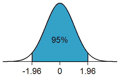
Similarly, the Confidence ellipses in PCA, PCoA, PLS-DA, and NMDS mark confidence intervals, which are descriptions of sample distributions that indicate that for any given sample that fits the population distribution, the probability of falling in a given interval is 95%. However, it should be noted that we are partially sampling the data and using the sampled data to represent the overall data distribution characteristics, so the number of samples will affect the estimation of the overall distribution. The more samples being sampled, the better the fitting of the overall distribution.

Q：What is permutation test

A：In statistics, part of the sample data of the research object is collected to describe the whole object. The more samples being collected, the more accurate the description of the whole, but in practice, the number of samples collected is often limited.Therefore, permutation tests are used when the number of samples collected is small and the distribution is unknown.

The permutation test was originally proposed by Fisher in the 1930s and is essentially a resampling method. It randomly samples all (or part) of the sample data, and then compares the sample statistics obtained by sampling with the actual observed sample statistics. Through a large number of permutations (default 999 times in R), it calculates the probability that the statistics after the permutation is greater than the actual observed statistics, which is the p value of the permutation test. Statistical inferences are made based on p values.

Note

Because the permutation test is random sampling, the results of multiple permutation tests are not completely consistent.

Reference

---

1. Dodge, Y., Cox, D., & Commenges, D. (2006). The Oxford Dictionary of Statistical Terms. Oxford University Press. ↩︎

2. Whittaker, R. H. (1960). Vegetation of the Siskiyou Mountains, Oregon and California. Ecological Monographs, 30(3), 279–338. https://doi.org/10.2307/1943563 ↩︎

3. Legendre, P., & Legendre, L. (2012). Numerical ecology (Third English edition). Elsevier. ↩︎

4. Bray, J. R., & Curtis, J. T. (1957). An Ordination of the Upland Forest Communities of Southern Wisconsin. Ecological Monographs, 27(4), 325–349. https://doi.org/10.2307/1942268 ↩︎

5. Jolliffe, I. T., & Cadima, J. (2016). Principal component analysis: A review and recent developments. Philosophical Transactions of the Royal Society A: Mathematical, Physical and Engineering Sciences, 374(2065), 20150202. https://doi.org/10.1098/rsta.2015.0202 ↩︎

6. Hefner, R. (1959). Warren S. Torgerson, Theory and Methods of Scaling. New York: John Wiley and Sons, Inc., 1958. Pp. 460. Behavioral Science, 4(3), 245–247. https://doi.org/10.1002/bs.3830040308 ↩︎

7. Kenkel, N. C., & Orloci, L. (1986). Applying Metric and Nonmetric Multidimensional Scaling to Ecological Studies: Some New Results. Ecology, 67(4), 919–928. https://doi.org/10.2307/1939814 ↩︎

8. Clarke, K. R. (1993). Non-parametric Multivariate Analyses of Changes in Community Structure. Australian Journal of Ecology, 18(1), 117–143. https://doi.org/10.1111/j.1442-9993.1993.tb00438.x ↩︎

9. Stat, M., Pochon, X., Franklin, E. C., Bruno, J. F., Casey, K. S., Selig, E. R., & Gates, R. D. (2013). The Distribution of the Thermally Tolerant Symbiont Lineage (symbiodinium Clade D) in Corals from Hawaii: Correlations with Host and the History of Ocean Thermal Stress. Ecology and Evolution, 3(5), 1317–1329. https://doi.org/10.1002/ece3.556 ↩︎